Structural Nested Mean Models for Causal Inference

Oisín Fitzgerald, January 2021

Causal inference considers questions such as: what would be the impact of giving someone a particular drug? There is a sense of action in a causal question, we are going to do something (hence Pearl's do notation (Pearl, 2009)). An associational question on the other hand, would ask: what is the most likely outcome of someone who is receiving a particular drug? It is passive (but still useful - e.g. predictive modelling). It is generally not the case that the answers to causal and associational questions will be the same, they can even lead to seemingly conflicting results. Most medical research asks a causal question; we wish to inform decisions. It is important we use the appropriate causal methods and thinking to answer the causal, rather than associational question (see Hernan and Robins (2020) for an in-depth treatment of this issue). There are many important considerations in answering causal questions from whether the question is worth answering, to what data needs to be collected (see Ahern (2018) for a good outline). This post considers arguably the least important aspect - the statistical methodology used to estimate the causal model parameters. I'll outline (as I poorly understand it) G-estimation of structural nested mean models (SNMM) for a single timepoint and two treatment options, and show some simulations using R along the way. First a brief review of the potential outcomes framework, those familiar with it can skip to the next section.

Potential outcomes framework

Within the potential outcomes framework causal inference becomes a missing data problem. For the case of two treatment levels $A \in \{0,1\}$ there are two potential outcomes $Y(1)$ and $Y(0)$ . If someone gets $A=0$ then the observed outcome is $Y=Y(0)$ (referred to as consistency), and $Y(1)$ is the counterfactual. That we only observe one potential outcome per person at a given time is referred to as the fundamental problem of causal inference (Holland, 1986). Our focus in this article will be calculating the conditional average treatment effect (CATE) $\tau(h) = E(Y(1)-Y(0)|H=h)$ where $H$ is a vector of effect modifiers.

To answer causal questions in a given dataset we require knowledge (or must make assumptions about) about the data generating process - in particular aspects of the treatment decision process (why did the clinical give patient A a particular drug?) and the outcome process (what is it about patient A that increases their risk of a particular outcome?). This knowledge allows us assess whether we can assume conditional exchangeability (unconfoundedness)

Y(a) \perp A |H=h

that within strata of $H$ we can consider treatment to have been randomly assigned, and positivity, that there exists some possibility that each patient could have received either treatment

P(A=a|H=h) > 0 \text{ for all values of }h

Conditional exchangeability will be key to constructing our estimation process and clarifies the difference between causal and associational analysis. To see this consider the canonical confounding example where sicker patients are more likely to get treated with a particular medicine (figure 1). A naive estimate of the difference $E(Y|A=1) - E(Y|A=0)$ may lead to the impression that treatment is harmful. However, if the treatment decision has been based on an illness severity factor, denoted by the random variable $X_1$ , that combines all factors predictive of the disease outcome then we have a biased result

E(Y|A=1) - E(Y|A=0) \ne E(Y(1) - Y(0))

In our example, only by accounting for $X_1$ can we get an unconfounded case where conditional exhangeability holds and the previous inequality becomes an equality.

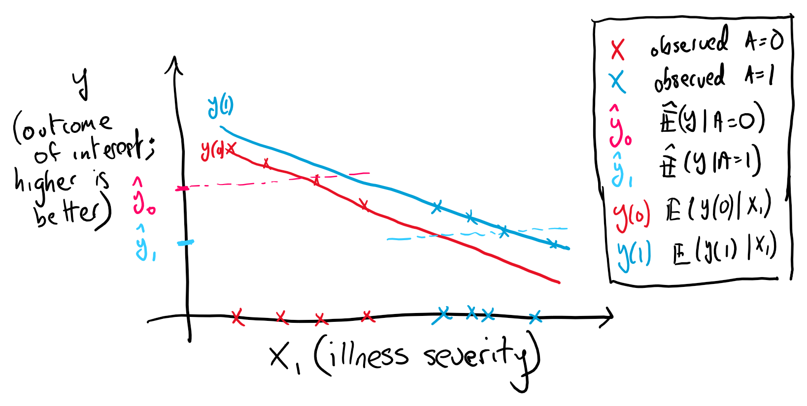
Figure 1. Illustration of confounding. The more severely ill (high X1) are more likely to get treated leading to the situation where the average outcome is worse in the treated. Notice that positivity is violated in this illustration.

In summary, we will need to make certain assumptions (1) consistency (2) unconfoundedness and (3) positivity around the data generating process (often reasonable but unverifiable) in order to be able to calculate an unbiased treatment difference. For an in-depth treatment see Hernan and Robins (2020).

G-methods Family

Not all statistical approaches that work for treatment comparison at a single timepoint generalise to situations involving time-varying treatments (where there is treatment confounder feedback). The G (generalised) methods, developed by James Robins and colleagues - including structural nested mean models (SNMMs), marginal structural models and G-computation, apply in both single and multi-stage treatment effect estimation (see references). If we want to compare the effectiveness of two treatment regimes or policies (e.g. intensive versus standard blood pressure control) using an observational sources such as electronic medical records the G-methods are an obvious choice. Here, we describe SNMMs and G-estimation in the context of a single treatment where there are a large number of competing approaches.

Structural Nested Mean Models

Structural nested mean models (SNMMs) are models for the contrast (mean difference) of two treatment regimes. This difference can be conditional on a set of effect modifying covariates. The term 'structural' indicates that they are causal models, and in a longitudinal setting the model takes a 'nested' form. Assume we observe a dataset $Z = (H,Y,A)$ where $H$ is a random variable indicating a patient history (covariates; e.g. blood pressure), $h_n$ is a realisation of $H_n$ for individual $n \in \{1,...,N\}$ , $Y$ is the outcome of interest and $A$ is the treatment indicator. In the single timepoint setting SNMMs involves fitting a model for the CATE

\tau(h) = E[Y(1)-Y(0)|H=h]

where $Y(a)$ is the potential outcome under treatment $A=a$ and the variables $X$ are effect modifiers. In particular we will discuss linear single timepoint SNMMs, where $h_n$ indicates a individual patients treatment history and $\phi$ a possible transformation of the original data (e.g. spline) resulting in a vector $\phi(h_n)$ of length $J$

\tau(h_n) = \sum_{j=1}^J \alpha_j \phi(h_n)

Within medicine it is generally considered reasonable to assume the effect modifying variables $H'$ are generally a subset of the history $H$ , with the dimension of $H'$ , $|H'|$ possible far smaller than $|H|$ . While a large numbers of factors - genetic, environmental and lifestyle - may influence whether someone develops a particular disease their impact on the effectiveness of a particular treatment may be neglible or noisy (effect modification is a higher order effect) in finite sample. Nevertheless, for simplicity of notation we will assume $H'=H$ from hereon.

There are several reasons we might be interested in only estimating the treatment contrast versus the outcome model $E(Y(a)|H=h,A=a)$ under each treatment directly. One way to think about the observed outcome $Y$ is as being composed of two components, a prognostic component and a predictive component. The prognostic component determines an individuals likely outcome given a particular medical history, and the predictive component determines the impact of a particular treatment. We can separate the expected outcome for a patient into these components

\begin{aligned} E[Y|A=a,H=h] &= E[Y|H=h,A=0] + E[Y(a) - Y(0)|H=h] \\ &= m_0(h) + \gamma(a,h) \tag{3} \end{aligned}

where the setting $A=0$ in $m_0$ corresponds to a control or baseline case. In many cases $m_0(h)$ may be a more complex function than $\tau(x) = \gamma(1,h)$ (Hahn, Murray & Carvalho, 2020). The potential for misspecification of $m_0(h)$ or desire for more parsimonious model motivates attempting to directly model $\tau(h)$ . If the final model will be used in practise, and must be explainable to subject matter experts, since empirically $\tau(h)$ may be simpler there may be large improvements in interpretability if we model $\tau(h)$ rather than an alternative. The parameter set $\psi$ of $\tau(h)$ is estimated using G-estimation, which we turn to next.

A Review: Independence and Covariance

G-estimation builds upon some basic some facts about conditional independence and covariances which we briefly review. The conditional independence of $X$ and $Y$ given $Z$ is denoted as $X \perp Y |Z=z$ . For probability densities $p$ this translates to $p(x,y|z) = p(x|z)p(y|z)$ . A direct result of this is that the conditional covariance of $X$ and $Y$ given $Z$ is equal to zero.

\begin{aligned} \text{Cov}(X,Y|Z) &= E[(X - E[X|Z])(Y - E[Y|Z])|Z] \\ &= E[XY|Z] - E[X|Z]E[Y|Z] \\ &= E[X|Z]E[Y|Z] - E[X|Z]E[Y|Z] \\ &= 0 \end{aligned}

Where the third line follows from the ability to factorise the conditional densities $E[XY|Z] = \int \int xy p(xy|z)dxdy = \int x p(x|z) dx \int y p(y|z)dy$ . We also note that 1) this holds if we replace $X$ or $Y$ by a function $f$ of $X$ or $Y$ and $Z$ , for example $f(X,Z) = X - E(X|Z)$ and 2) relatedly that $E[X(Y - E[Y|Z])|Z] = 0$ .

G-Estimation

G-estimation is an approach to determining the parameters of a SNMM. As we are modelling a treatment contrast in a situation where only one treatment is observed per individual we need a method that accounts for this missingness. There are two explanations below, the second is more general, with some repitition.

Explanation 1: Additive Rank Preservation

One approach to explaining G-estimation is through assuming additive rank preservation with regard to the treatment effect (Hernan & Robins, 2020). Additive rank preservation is the assumption that the treatment effect is the same for everyone, that $Y(1)-Y(0) = \psi_0$ . We emphasise that this is at the individual level (see figure 2). As shown later it is not a requirement for G-estimation that this assumption holds, it is expository tool.

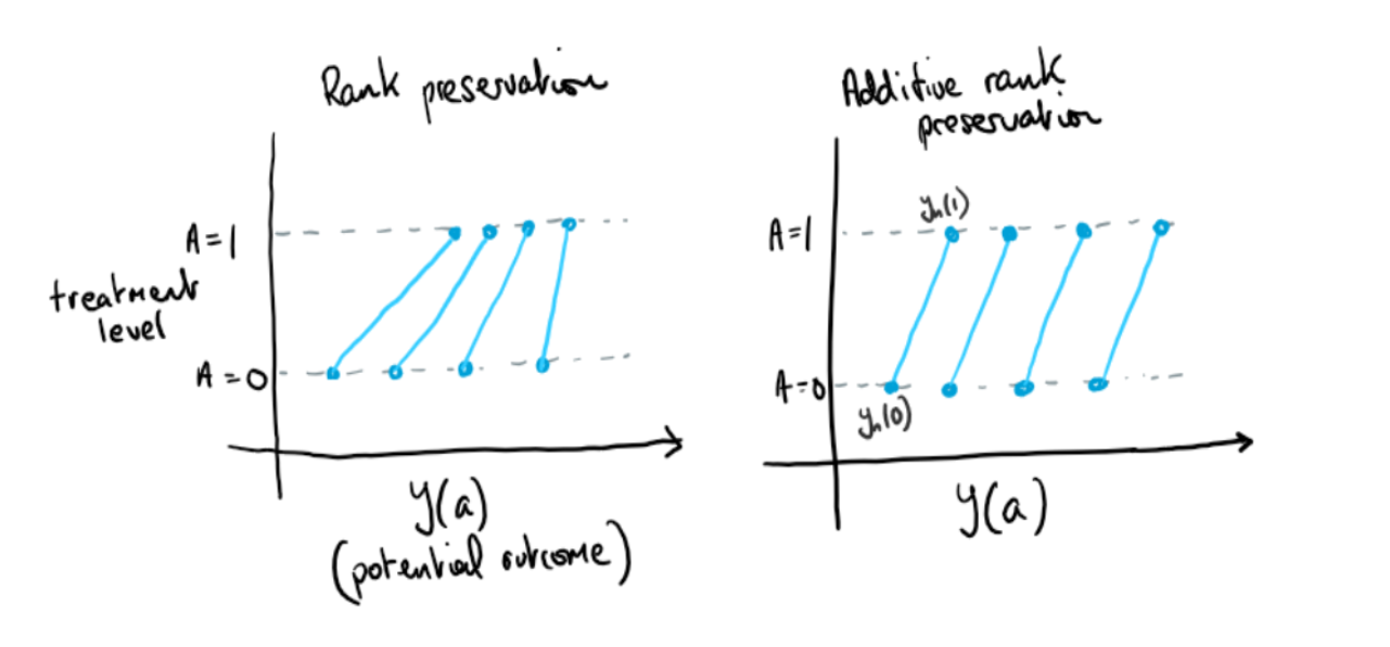
Figure 2. Illustration of additive and nonadditive rank preservation

Notice that for the case of additive rank preservation with no effect modification the following holds

\begin{aligned} Y(0) &= Y - A[Y(1)-Y(0)] \\ Y(0) &= Y - A\psi \\ \end{aligned}

If we call this final expression $G(\psi) = Y - A\psi$ then utilising the assumption of unconfoundedness $Y(a) \perp A|H=h$ this should be uncorrelated with any function $S(A)$ of the treatment assignment mechanism, conditional on the confounders $H$ . For this case of no effect modification we'll let $S(A) = A$ (we'll return to choice of $S$ later). We then have the estimating equation $U(\psi;H,A) = \sum_{n=1}^N G_n(\psi)[A_n - E(A_n|X_n)] = 0$ . For the cases where $E(A_n|H_n = h_n)$ is unknown we replace it with an estimate. This equation can then be solved for the unknown $\psi$ , giving us an approach towards estimation. We continues this case below in Example 1.

Explanation 2: More General Case

Now consider the more general case where $\psi$ is a vector of parameters of our SNMM $\tau_{\psi}(h) = E(Y(1)-Y(0)|H=h)$ . Our analog of $G(\psi)$ is now equal to $Y(0)$ in expectation

\begin{aligned} E(G(\psi)|H) &=E[Y - A(Y(1)-Y(0))|H] \\ &= E[Y|H] - E[A(Y(1)-Y(0))|H] \\ &= E[AY(1) + (1-A)Y(0)|H] - E[A(Y(1)-Y(0))|H] \\ &= E[Y(0)|H] \end{aligned}

Where we make use of the consistency assumption $Y = AY(1) + (1-A)Y(0)$ in going from line two to three. As a result we have the following estimating equation $U(\tau;A_n,H_n) = \sum_{n=1}^N G_n(\psi)(S(A_n,H_n)-E[S(A_n,H_n)]) = 0$ for the general case in a single stage setting which is zero in expectation $E(U|L) = 0$ . Note that we could mean center $G(\psi)$ which we will return to. For the case where $\tau_{\psi}(h)$ can be expressed as a linear model this can be explicity solved, we outline this case below in Example 2.

Some examples

Example 1

In the case of $\tau(h) = \psi_0$ (the average treatment effect (ATE)), i.e. $G(\psi_0) = Y - \psi_0A$ and $S(A) = A$ we have an explicit solution

\begin{aligned} U(\psi_0;H,A) &= 0 \\ \sum_n^N G(\psi_0) [A - E(A_n|H_n=h_n)] &= 0 \\ \sum_n^N [Y_n - \psi_0A_n] [A_n - E(A|H_n)] &= 0 \\ \psi_0 = \sum_n^N \frac{Y_n[A_n - \pi(h_n)]}{\sum_n^N A_n [A_n - \pi(h_n)]} \end{aligned}

As mentioned, in observational studies where the treatment assignment mechanism is unknown we replace $\pi(h_n) = E(A|H_n=h_n)$ (the propensity score) with an estimate, using e.g. logistic regression or more complex models.

Let's simulating this situation for a data generating model of the form

\underline{\text{Simulation 1 settings}} \\ E(Y(a)|H_1=h_1,A=a) = -1.4 + 0.8h_1 + \tau_0a + \epsilon \\ \tau_0 = 2.5\\ \epsilon \sim \text{Normal}(0,1) \\ H_1 \sim \text{Uniform}(-0.5,3.0)\\ P(A=1|H_1=h_1) = (1 + \text{exp}(2 - 1.8h_1)^{-1}\\

Notice observations with larger values of $H_1$ are more likely to be treated. We'll compare fitting a SNMM for the parameter $\tau_0$ with fitting an linear model for the full conditional expectation. The simulation set up is adapted from Chakraborty and Moodie (2013). As shown in figure 3 both methods return similar results. This is to be expected; the advantage of SNMMs and G-estimation is primarily in situations where the prognostic component $m_0(h)$ is complex and we want a parsimonious model (we show this case below), and in time-varying treatment setting (in part 2).

## SIMULATION 1
M <- 500 # number of rins
tauM <- replicate(M, {
  N <- 100
  # generate data
  h1 <- runif(N,-0.5,3)
  ps <- function(x) 1/(1 + exp(2 - 1.8*h1))
  a <- 1*(ps(h1) < runif(N))
  y <- -1.4 + 0.8*h1 + 2.5*a + rnorm(N)
  # estimate probability of treatment
  pm <- glm(a ~ h1,family = binomial())
  ph <- fitted(pm)
  w <- (a-ph)
  # estimate treatment effect
  tauh_g <- sum(w*y)/sum(a*w)
  tauh_lm <- lm(y ~ h1 + a)$coef["a"]
  c(tauh_g,tauh_lm)
})

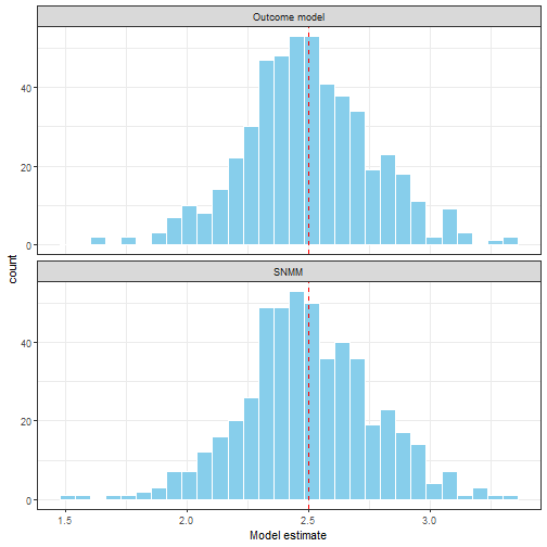
A comparison of OLS estimation of the outcome model E(Y|A,H) and G-estimation of the SNMM

Figure 3. A comparison of OLS estimation of the outcome model E(Y|A,H) and G-estimation of the SNMM

Example 2

Now consider the case where $\tau(h)$ is a function of several variables. Our decision rule for which treatment to use must consider several variables. We can model this using a linear model with covariates $\tau(h_n) = \psi_0 + \sum_{k=1}^K\psi_k h_{kn}$ . The resulting empirical estimating equation is

\begin{aligned} U(\psi;A_n,H_n) &= \sum_{n=1}^{N}G(\psi)[S(A_n,H_n)-E(S(A_n,H_n)|H_n)] \\ U(\psi;A_n,H_n) &= \sum_{n=1}^{N}[Y_n - (\psi_0 + \sum_{k=1}^K\psi_k h_{kn})][S(A_n,H_n)-E(S(A_n,H_n)|H_n)] \\ \end{aligned}

Here we have replaced $S(A_n)$ with $S(A_n,H_n)$ which changes nothing as $H_n$ is treated as a constant. As stated this appears to be a single equation with $K+1$ unknowns. However, as $S(A_n,H_n)$ is an 'arbitrary' function we can convert it into $K+1$ equations through choosing $S(A_n,H_n)$ to be the vector valued function $S(A_n,H{*n}) = (1,h_1,,...h_K)^t\cdot A_n$ . This gives $K+1$ estimating equations

\begin{aligned} U_1(\psi;A_n,H_n) &= \sum_{n=1}^{N}[Y_n - (\psi_0 + \sum_{k=1}^K\psi_k x_{kn})][A_n-\pi(h_n)] \\ U_2(\psi;A_n,H_n) &= \sum_{n=1}^{N}[Y_n - (\psi_0 + \sum_{k=1}^K\psi_k x_{kn})][A_n-\pi(h_n)] h_{1n} \\ \dots \\ U_K(\psi;A_n,H_n) &= \sum_{n=1}^{N}[Y_n - (\psi_0 + \sum_{k=1}^K\psi_k x_{kn})][A_n-\pi(h_n)] h_{Kn} \\ \end{aligned}

In order to write the above estimating equations in matrix/vector form let $\textbf{H}$ be our $n \times (K+1)$ effect modifier/confounder design matrix, $\textbf{A} = \text{diag}(A_1,A_2,\dots,A_N)$ and $\textbf{W} = \text{diag}(A_1-\pi(h_1),\dots,A_N-\pi(h_N))$ . Then our $K+1$ estimating equations in matrix/vector form are $\textbf{U}(\psi;A_n,H_n) = \textbf{H}^t\textbf{W}(\textbf{y}-\textbf{A}\textbf{H}\boldsymbol{\psi})$ . Solving for $\boldsymbol{\psi}$ gives

\begin{aligned} \boldsymbol{\psi} &= (\textbf{H}^t\textbf{W}\textbf{A}\textbf{H})^{-1}\textbf{H}^t\textbf{W}\textbf{y} \end{aligned}

Simulating this situation, again building the settings off Chakraborty and Moodie (2013), we have two settings, with the $m_0$ component (3) alternatively linear and non-linear. The treatment effect component $\tau(h)$ is always linear - we'll come to non-linar $\tau(h)$ next.

\underline{\text{Simulation 2 settings}} \\ \text{linear case:}\hspace{5 mm}E(Y(a)|H_1=h_1,A=a) = -1.4 + 0.8h_1 + \psi_0 a + \psi_1 a h_1 + \epsilon \\ \text{nonlinear case:}\hspace{4 mm}E(Y(a)|H_1=h_1,A=a) = -1.4h_1^3 + e^{h_1} + \psi_0 a + \psi_1 a h_1 + \epsilon \\ \text{(all other setting as simulation 1)}

We compare G-estimation of the SNMM with a (linear) outcome model for the full expectation $E(Y|H,A)$ . While this shows the strength of SNMM in avoiding misspecification it is not entirely fair, as in an empirical setting a simple plot of the data would reveal that a linear model is a bad idea.

gest_snmm <- function(X,y,a,ph) {
  w <- (a-ph)
  W <- diag(w)
  A <- diag(a)
  t1 <- solve(t(X) %*% W %*% A %*% X)
  t2 <- t(X) %*% W %*% y
  t1 %*% t2
}

## SIMULATION 2
M <- 500  # number of runs
tauM <- replicate(M, {
  # generate data for linear and non-linear cases
  N <- 100
  h1 <- runif(N,-0.5,3)
  ps <- function(x) 1/(1 + exp(2 - 1.8*h1))
  a <- 1*(ps(h1) < runif(N))
  psi0 <- 2.5
  psi1 <- 1.5
  y1 <- -1.4 + 0.8*h1 + psi0*a + psi1*a*h1 + rnorm(N)
  y2 <- -1.4*h1^3 + exp(h1) + psi0*a + psi1*a*h1 + rnorm(N)
  # estimate probability of treatment
  pm <- glm(a ~ h1,family = binomial())
  H <- cbind(rep(1,N),h1)
  ph <- fitted(pm)
  # estimate treatment effect
  g1 <- as.vector(gest_snmm(H,y1,a,ph))
  g2 <- as.vector(gest_snmm(H,y2,a,ph))
  ols1 <- lm(y1 ~ h1 + a + h1*a)$coef[c("a","h1:a")]
  ols2 <- lm(y2 ~ h1 + a + h1*a)$coef[c("a","h1:a")]
  c(g1,g2,ols1,ols2)
})

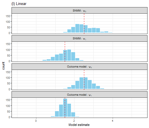
A comparison of OLS estimation of the outcome model E(Y|A,H) and G-estimation of the SNMM for a linear outcome model.

Figure 4. A comparison of OLS estimation of the outcome model E(Y|A,H) and G-estimation of the SNMM for a linear outcome model.

A comparison of OLS estimation of the outcome model E(Y|A,H) and G-estimation of the SNMM for a non-linear outcome model.

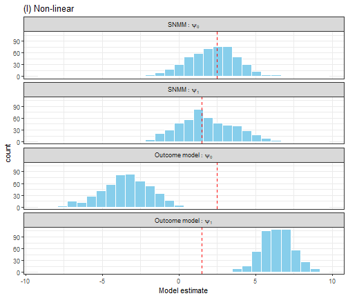
Figure 5. A comparison of OLS estimation of the outcome model E(Y|A,H) and G-estimation of the SNMM for a non-linear outcome model.

More efficient G-estimation

Returning to the idea that setting $U(\psi) = 0$ follows from $\text{Cov}(Y(0),S(A,H)|H) = 0$ , it turns out there is a more efficient form of G-estimation if we take full advantage of this equality. As per Wikipedia "a more efficient estimator needs fewer observations than a less efficient one to achieve a given performance".

Above we use an empirical version of $E(Y(0)(A-S(A|H))|H)=0$ as out estimating equation. That is because we don't know $E(Y(0)|H)$ . However, we can estimate it; to do this fit a model and use it to predict $\hat{m}_0(h) = E(Y(0)|H)$ for all observations. Then rather than using $y$ in our estimation procedures we use $\tilde{y} = y-\hat{m}_0(h)$ . The need to estimate several models before G-estimation may seem to add the number of possible sources of error however it actually has the opposite impact. This approach is doubly robust, meaning that if either x or y are correctly specified then the estimated causal effect is unbiased. Correct specification refers to the function form of the model, e.g. aspects such as linear/non-linear effects and interactions. Failure to include confounders would lead to bias even if the model was "correct" for the measured confounders. For our linear model, with m being, the doubly robust estimate is

\begin{aligned} \hat{\boldsymbol{\psi}}_e &= (\textbf{H}^t\textbf{W}\textbf{A}\textbf{H})^{-1}\textbf{H}^t\textbf{W}(\textbf{y}-\hat{m}_0) \end{aligned}

What is the intuition behind this? We can think of it as information simplification - by taking out $m_0(h)$ we are allowing the estimation to focus on changes with $H$ for $A=0$ is informative about what variation is not due to the treatment effect. Generally noise reduction $\rightarrow$ signal enhancement. For a more detailed argument see Athey and Imbens (2019) or Nie and Wager (2017). We can still use our avoid function gest_snmm for efficient G-estimation, but rather than passing in the actual y we pass in $\tilde{y} = y - E(Y|A=0,H=h)$ which we can estimate using an approach of choice.

Non-linear effect modification

So far we have talked about and simulated linear $\tau(h)$ , but what if the effect modification is non-linear? Restricting ourselves to linear models in the age of machine learning seems so uncool. I'll add that many of the ideas underlying G-estimation and snmm come up in gradient trees (Athey 2019) or R-learning (Nie & Wager 2017). As a first step towards non-linear models for $\tau$ we'll consider approaches that involve transformations of the design matrix $H$ (the matrix containing our effect modifiers and generally a vector of 1s for the main (first order) effect of treatment). So we have a transformation $\Phi: \mathbb{R}^{n \times p} \to \mathbb{R}^{n \times q}$ , including methods such as the Fourier transform, polynomial expanstions, spline basis matrices. We then replace $X$ with $\Phi(H)$ in our estimation procedure

\begin{aligned} \hat{\boldsymbol{\psi}}_e &= (\boldsymbol{\Phi}^t\textbf{W}\textbf{A}\boldsymbol{\Phi})^{-1}\boldsymbol{\Phi}^t\textbf{W}(\textbf{y}-\hat{m}_0) \end{aligned}

To illustrate this, lets do another simulation. In this case $\tau$ is non-linear.

\underline{\text{Simulation 3 settings}} \\ tau(h_1,h_2) = \psi_0 + 0.7 e^{h1} + 0.5h_2 + 0.4 h_2^2 + \epsilon_1 \\ E(Y(a)|H=h,A=a) = 1.2h_2 - 1.4h_2^2 + 0.8e^{h_1} + a\tau(h) + 3\epsilon_2 \\ \psi_0 = 2.5 \\ \psi_1 = 1.5 \\ H_1 \sim \text{Uniform}(-0.5,3) \\ H_2 \sim \text{Normal}(2,3) \\ \epsilon_1,\epsilon_2 \sim N(0,1) \\ P(A=1|H=h) = (1 + \text{exp}(2 - 1.8h_1 + 0.2h_2)^{-1}\\

We have increased the number of variables to two (clearly the simulations should not be relied upon!). For this simulation I've increased the sample size to $N=1000$ .

## SIMULATION 3
M <- 500  # number of runs
tauM <- replicate(M, {
  # generate data
  N <- 1000
  x1 <- runif(N,-0.5,3)
  x2 <- rnorm(N,2,3)
  ps <- function(x1,x2) 1/(1 + exp(2 - 1.8*x1 + 0.2*x2))
  a <- 1*(ps(x1,x2) < runif(N))
  psi0 <- 2.5
  psi1 <- 1.5
  tau <- psi0 + 0.7*exp(x1) + 0.5*x2 + 0.4*x2^2 + rnorm(N)
  y <- 1.2*x2 - 1.4*x2^2 + 0.8*exp(x1) + a*tau + rnorm(N,sd = 3)
  # estimate probability of treatment
  pm <- glm(a ~ x1 + x2,family = binomial())
  Xs <-  cbind(rep(1,N),bs(x1),bs(x2))
  ph <- fitted(pm)
  # estimate treatment effect
  ols <- lm(y ~ bs(x1) + bs(x2) + a + bs(x1)*a + bs(x2)*a)
  df0 <- data.frame(x1,x2,a=0)
  df1 <- data.frame(x1,x2,a=1)
  tau_ols <- predict(ols,df1) - predict(ols,df0)
  g <- gest_snmm(Xs,y - predict(ols,df0),a,ph)
  tau_g <- as.vector(Xs %*% g)
  c(bias_g=mean((tau_g-tau)),
    bias_l=(mean((tau_ols-tau))),
    mse_g=mean((tau_g-tau)^2),
    mse_l=(mean((tau_ols-tau)^2)))
})

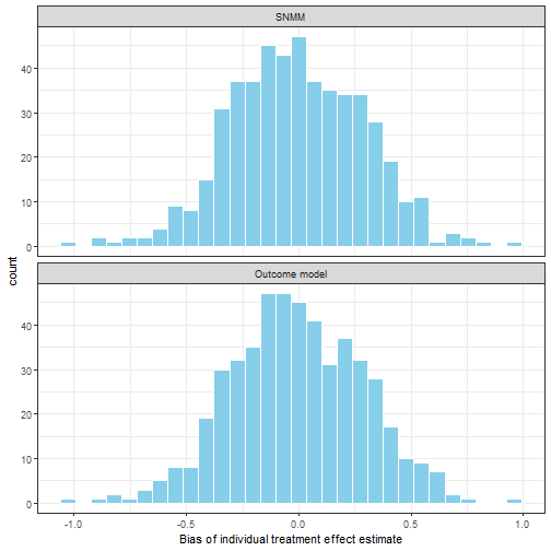
Average bias of individual treatment effect

Figure 6. Average bias of individual treatment effect

Average meas square error of individual treatment effect

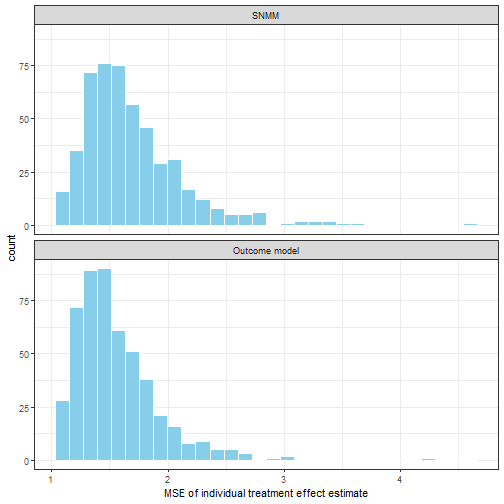
Figure 7. Average meas square error of individual treatment effect

Standard errors and confidence intervals

Quantifying uncertainty in our parameter estimates is important. For G-estimation of SNMMs the non-parametric bootstrap offers a general approach to estimation of standard errors, allowing incorporation of the uncertainty arising from estimating $\pi(h)$ and $m_0(h)$ .

Conclusion and up-next

We've outlined the linear SNMM and G-estimation, focusing on the single stage setting. While SNMM are not often used in practise I hope that as we go through this series their strengths will become clear. We have largely dealt with simplistic situations in which the CATE is of interest to emphasise the fundamentals of the method. G-estimation is based on setting an empirical covariance equal to zero building off the assumptions from causal inference - ignorability/unconfoundedess, consistency and positivity. As mentioned at the beginning there is much more to causal inference than the methods and often subject matter knowledge plays an important role in justifying the reasonableness of these assumptions and designing the data collection/extraction process.

There are several things we haven't covered in this tour of SNMM and G-estimation:

Non-continous outcomes - in particular binary outcomes
More than point estimates - quantiles or distributions
Treatments that vary over time
Simulations that really test SNMM (or it's competitors) in the complex and noisy datasets common in data science practise

We'll come back to these topics, in particular time varying treatments in subsequent posts. Thanks for reading.

Thanks to Oscar Perez Concha for reading and discussing drafts of this.

Reading and links

Ahern, Jennifer. 2018. Start with the ’c-Word,’ Follow the Roadmap for Causal Inference. American Public Health Association.
Athey, Susan, Julie Tibshirani, Stefan Wager, and others. 2019. Generalized Random Forests. The Annals of Statistics 47 (2): 1148–78.
Chakraborty, Bibhas, and Erica EM Moodie. 2013. Statistical Methods for Dynamic Treatment Regimes: Reinforcement Learning, Causal Inference, and Personalized Medicine. Springer.
Hahn, P Richard, Jared S Murray, Carlos M Carvalho, and others. 2020. Bayesian Regression Tree Models for Causal Inference: Regularization, Confounding, and Heterogeneous Effects. Bayesian Analysis.
Hernan, Miguel A, and James M Robins. 2020. Causal Inference: What If?” Boca Raton: Chapman & Hall/CRC
Holland, Paul W. 1986. Statistics and Causal Inference. Journal of the American Statistical Association 81 (396): 945–60.
Nie, Xinkun, and Stefan Wager. 2017. Quasi-Oracle Estimation of Heterogeneous Treatment Effects. arXiv Preprint arXiv:1712.04912.
Pearl, Judea, and others. 2009. Causal Inference in Statistics: An Overview. Statistics Surveys 3: 96–146.
Robins, James. 1986. A New Approach to Causal Inference in Mortality Studies with a Sustained Exposure Period—Application to Control of the Healthy Worker Survivor Effect. Mathematical Modelling 7 (9-12): 1393–1512.
Robins, James M, Donald Blevins, Grant Ritter, and Michael Wulfsohn. 1992. G-Estimation of the Effect of Prophylaxis Therapy for Pneumocystis Carinii Pneumonia on the Survival of Aids Patients. Epidemiology, 319–36.
Robins, James M, Miguel Angel Hernan, and Babette Brumback. 2000. Marginal Structural Models and Causal Inference in Epidemiology. LWW.
Vansteelandt, Stijn, Marshall Joffe, and others. 2014. Structural Nested Models and G-Estimation: The Partially Realized Promise. Statistical Science 29 (4): 707–31.

A data science blog